The 5 Dimensions of Parallelism

08 Nov, 2026

A little while ago, I gave a talk at an Google event on a topic that eats up an unreasonable amount of my waking hours: how you take a language model that has no business fitting on a single graphics card and stretch it across tens, hundreds, or thousands of GPUs without setting your cluster—or your cloud budget—on fire.

After the talk, a bunch of folks came up asking for the slides. I always hesitate to just drop a raw slide deck on LinkedIn. Slides are meant to be a visual backdrop while somebody is talking; when you read them cold, half the nuance is missing and they just look like boxes and arrows. So instead of dumping a PDF link and calling it a day, I sat down and wrote out the entire talk as a long-form post—walking through every slide, the actual matrix math behind the cuts, and the practical systems trade-offs that didn't fit on a 30-minute stage timer.

Grab a coffee. This is a long read.

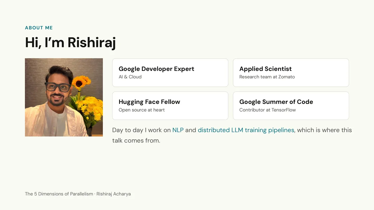
Quick intro if we haven't crossed paths before: I’m Rishiraj. I work as an Applied Scientist on the research team at Zomato, and outside of work I’m a Google Developer Expert (GDE) for AI & Cloud and a Hugging Face Fellow. I got my start in open source years ago contributing to TensorFlow during Google Summer of Code, and I’ve been hooked on the systems side of ML ever since.

My day job revolves around NLP and distributed LLM training pipelines. Everything in this post comes straight from the trenches of staring at nvidia-smi, hunting down silent NCCL hangs at 2 AM, and figuring out why a training script that hummed along happily at a 4K context length suddenly explodes when you bump it to 32K.

One Model, Five Ways to Cut It

Training a small model on a single GPU is peaceful. Your data sits on the card, your weights sit on the card, the forward pass goes up, the backward pass comes down, the optimizer steps, and you move on with your life.

The moment you try to train or fine-tune a modern LLM at scale, you slam into two walls:

1. The Memory Wall: The model weights, gradients, optimizer states, and intermediate activations simply do not fit in a single GPU’s VRAM.
2. The Time Wall: Even if your model does fit on one card, training it on billions or trillions of tokens on a single GPU would take years.

To get past both walls, you have to slice your training run across multiple GPUs. Distributed training papers love inventing intimidating names for their setups, which makes the field look way more fragmented than it actually is. Strip away the branding, and there are really only five ways to cut a model.

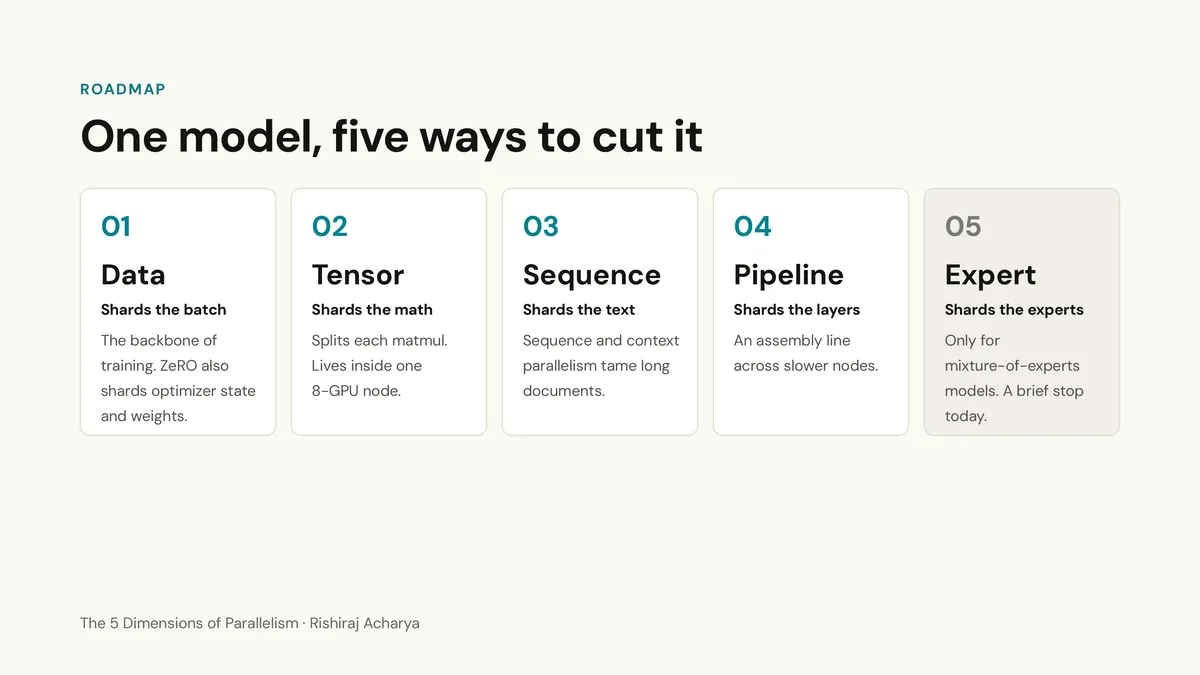
Here is the whole map:

1. Data Parallelism (DP): Shards the batch. Every GPU gets a different slice of data. When paired with ZeRO or FSDP, we also shard the optimizer states, gradients, and weights across those GPUs.
2. Tensor Parallelism (TP): Shards the math. We split individual matrix multiplications down the middle so multiple GPUs compute a single layer together in lockstep. This lives strictly inside one 8-GPU node.
3. Sequence & Context Parallelism (SP/CP): Shards the text. When sequences get long, we split the token dimension across GPUs so activation memory doesn't blow up.
4. Pipeline Parallelism (PP): Shards the layers. Server 1 takes layers 1 to 4, Server 2 takes layers 5 to 8, and they pass activations down the line like a factory assembly belt.
5. Expert Parallelism (EP): Shards the experts. Exclusive to Mixture-of-Experts (MoE) models, where different GPUs host different expert sub-networks and route tokens back and forth.

Those five dimensions aren't arbitrary software abstractions. They come directly from the tensor shapes of a Transformer.

Part 0: Foundations (Where Is All the VRAM Going?)

To see why there are only five cuts, trace a single batch of text as it flows through a standard decoder-only Transformer.

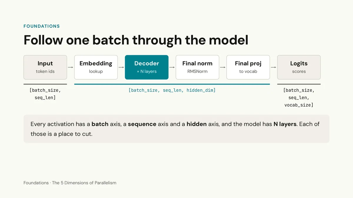
Your input enters the model as integer token IDs of shape [batch_size, seq_len]. The embedding lookup turns each token ID into a dense vector, giving you a 3D activation tensor of shape [batch_size, seq_len, hidden_dim]. That tensor passes through $N$ identical decoder layers, hits a final RMSNorm, and gets projected by the language modeling head into [batch_size, seq_len, vocab_size] logits.

Look at the activation tensor sitting in the middle of that diagram—[batch_size, seq_len, hidden_dim]—and the N layers it travels through. Every single dimension of parallelism is just a decision about which axis to slice:

• Slice batch_size $\to$ Data Parallelism
• Slice seq_len $\to$ Sequence / Context Parallelism
• Slice hidden_dim $\to$ Tensor Parallelism
• Slice N layers $\to$ Pipeline Parallelism
• Slice parallel MLP branches inside a layer $\to$ Expert Parallelism

For a long time, the standard playbook for big models was called "3D Parallelism," which meant combining the three classic cuts: Pipeline, Tensor, and Data.

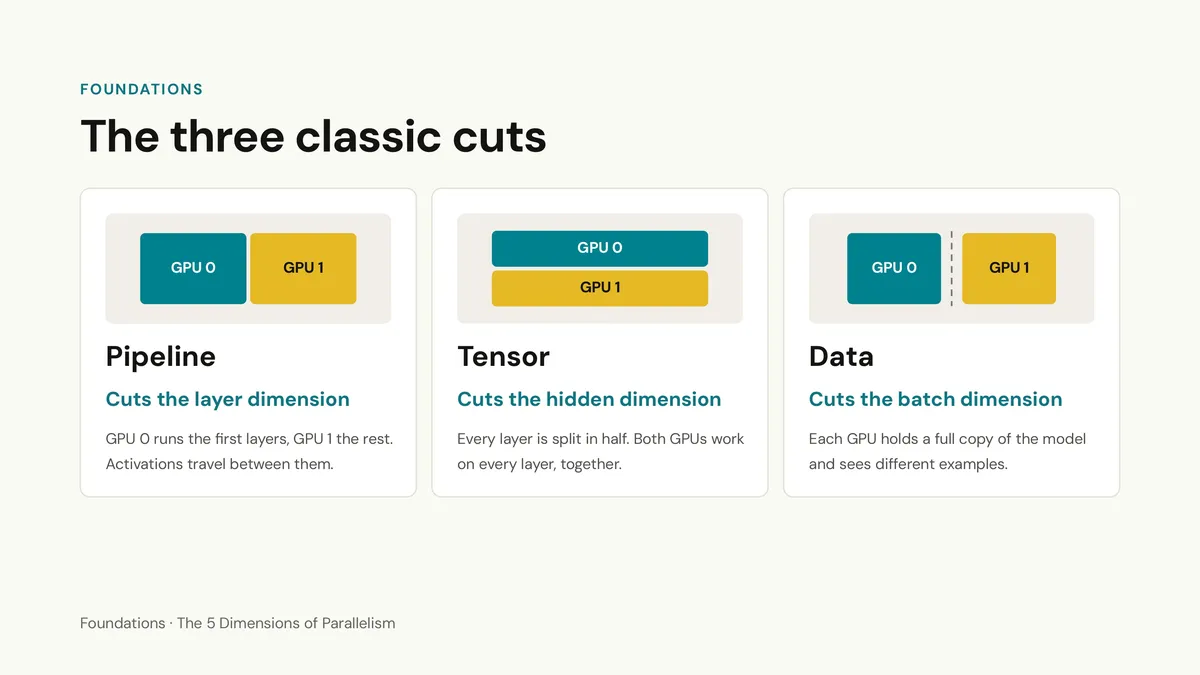
If you picture two GPUs sharing the work:

• Pipeline Parallelism cuts horizontally between layers. GPU 0 runs the early layers and hands the resulting activations to GPU 1, which runs the remaining layers.
• Tensor Parallelism cuts vertically through every layer. GPU 0 and GPU 1 work on Layer 1 at the exact same time—each doing half the matrix math—then sync up and move to Layer 2 together.
• Data Parallelism doesn't cut the model architecture at all. Both GPUs run the full model, but each looks at different training examples.

Before we start splitting models across a cluster, though, we need to do some back-of-the-envelope memory math. Most out-of-memory crashes happen because people underestimate how much state a training loop actually holds.

The 20-Byte Rule

Almost everyone who starts training LLMs makes the same mental calculation at least once: "I want to train an 8B parameter model in BF16. Two bytes per parameter times 8 billion is 16 GB. I have an 80 GB A100, so I've got 64 GB to spare."

Then you launch the script and it OOMs before finishing the first step.

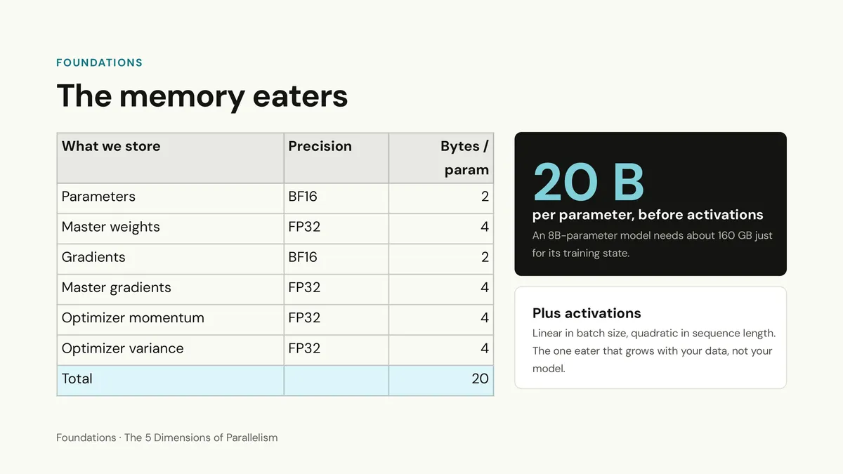
The 16 GB figure only accounts for inference weights. When you train with mixed precision and AdamW, here is what actually sits in memory for every single parameter:

• Parameters (BF16): 2 bytes. These are the weights used in the fast forward and backward matrix multiplications.
• Master weights (FP32): 4 bytes. In BF16, you only have 7 bits of mantissa. If your weight is $1.0$ and your learning rate times gradient update is $0.0001$, adding them in BF16 rounds right back to $1.0$—the model literally stops learning. So we keep a master copy of the weights in FP32 where small updates can accumulate accurately, and cast down to BF16 before each forward pass.
• Gradients (BF16): 2 bytes, produced during backprop.
• Master gradients (FP32): 4 bytes. Many distributed frameworks accumulate or reduce gradients in FP32 to avoid underflow/overflow across large reduction trees. (Even if your framework skips persistent FP32 master gradients, temporary buffers during reduction and optimizer steps often eat a similar chunk of peak memory, bringing the floor to 16–20 bytes).
• Optimizer momentum (FP32): 4 bytes for Adam's first moment ($m$).
• Optimizer variance (FP32): 4 bytes for Adam's second moment ($v$).

Add those up and you get 20 bytes per parameter. Multiply 20 bytes by 8 billion parameters, and your "16 GB" model actually needs 160 GB of VRAM just to hold its static training state—before a single token of training data ever touches the GPU.

And once data does touch the GPU, you have to pay for activations. During the forward pass, PyTorch has to save the intermediate outputs of every layer in memory because the backward pass needs them to compute gradients via the chain rule (for a linear layer $Y=XW$, computing the weight gradient $dW=X^{T}dY$ requires the original input activation $X$). Unlike weights and optimizer states, which are fixed by your model size, activation memory scales linearly with batch_size and explodes with seq_len.

Before you throw more GPUs at activation memory, there are two single-GPU techniques you should always turn on first.

Trick 1: Activation Recomputation (Gradient Checkpointing)

If saving every intermediate tensor from the forward pass is what fills up your VRAM, the fix is simple: stop saving all of them.

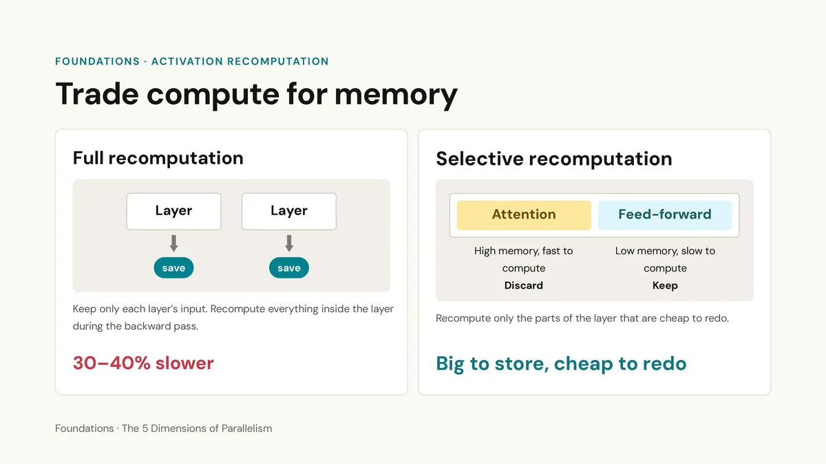
With activation recomputation (called gradient_checkpointing in Hugging Face and PyTorch), you only save the activation tensor at the input boundary of each Transformer layer and discard everything computed inside the layer. During the backward pass, right before backpropagating through Layer $k$, the GPU takes that saved input boundary tensor and re-runs Layer $k$’s forward pass on the fly to regenerate the internal activations it needs.

Doing full recomputation across every layer slashes activation memory from $O(\text{num\_layers}\times \text{internal\_ops})$ down to just the layer boundaries, at the cost of roughly 30–40% extra training time (since you are effectively running a second forward pass during backward).

If you want most of the memory savings without eating the full 35% compute hit, you use selective recomputation:

• Attention produces massive intermediate activations (especially pre-softmax scores or multi-head projections across long sequences), but thanks to modern fused kernels, recomputing it is relatively fast. So we discard its internals and recompute them in backward.
• Feed-Forward (MLP) blocks do heavy matrix multiplications (up, gate, down) that dominate the FLOPs of the model. Recomputing them is expensive, so we keep their activations in memory.

Trick 2: Gradient Accumulation

For stable optimization, LLMs want large effective batch sizes—often millions of tokens per step. Your GPU, meanwhile, might only be able to hold 1 or 2 sequences at a time without running out of activation memory.

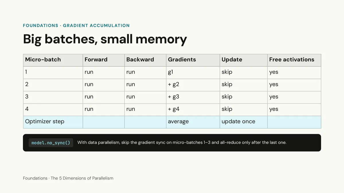
Gradient accumulation decouples your mathematical batch size from your physical memory footprint. Instead of feeding a batch of 4 all at once, you run 4 sequential micro-batches of size 1:

1. Run the forward and backward pass on Micro-batch 1. This populates your gradient buffers with $g_1$. As soon as backward finishes, PyTorch frees the forward activations for Micro-batch 1. You do not run the optimizer yet.
2. Run forward and backward on Micro-batch 2. PyTorch adds the new gradients directly into the existing buffer ($g_1+g_2$), and frees Micro-batch 2’s activations.
3. Do the same for Micro-batches 3 and 4.
4. Average the accumulated gradients $(g_1+g_2+g_3+g_4)/4$ and call optimizer.step() once.

You get the exact same weight update as a batch of 4, using only a quarter of the activation memory.

One classic footgun here: when you combine gradient accumulation with Data Parallelism, make sure micro-batches 1 through 3 are wrapped in PyTorch’s model.no_sync() context manager. By default, DDP hooks into the backward pass and triggers a network all-reduce every time loss.backward() finishes. If you forget no_sync(), your GPUs will pointlessly synchronize un-stepped partial gradients across the network on micro-batches 1, 2, and 3—wasting 75% of your network bandwidth.

Dimension 1: Data Parallelism (Sharding the Batch)

Data Parallelism is the workhorse of distributed training. In standard Distributed Data Parallel (DDP), every GPU holds a complete copy of the model, receives a different slice of the data batch, runs its own forward and backward pass, and then averages gradients across all GPUs via an all-reduce collective so every replica stays in sync.

If you coded this naively—wait for the whole backward pass to finish, call dist.all_reduce() on all gradients, wait for the network, then run the optimizer—your GPU utilization would tank. Your compute cores would sit idle during communication, and your network card would sit idle during computation.

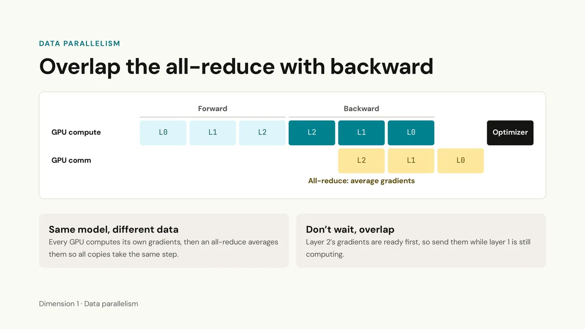
The saving grace of Data Parallelism is that backpropagation runs in reverse: Layer 2 (L2), then Layer 1 (L1), then Layer 0 (L0).

As soon as the backward pass finishes L2, the gradients for L2 are final. Nothing happening in L1 or L0 will alter them. So DDP groups gradients into buckets and fires off an asynchronous all-reduce on L2’s gradients over NCCL at the exact same time the CUDA compute stream moves on to calculating L1’s backward pass. By the time L0 finishes its backward pass, nearly all the network communication has already finished in the background.

ZeRO & FSDP: Stop Storing the Same Thing $N$ Times

Overlapping communication makes plain DDP fast, but DDP doesn't help at all with the Memory Wall. If your 8B model takes 160 GB of training state, and you have 8 GPUs with 80 GB each, plain DDP tries to put all 160 GB onto every single card. You have 640 GB of aggregate cluster memory, yet you still crash with an OOM because all 8 GPUs are hoarding identical copies of the same state.

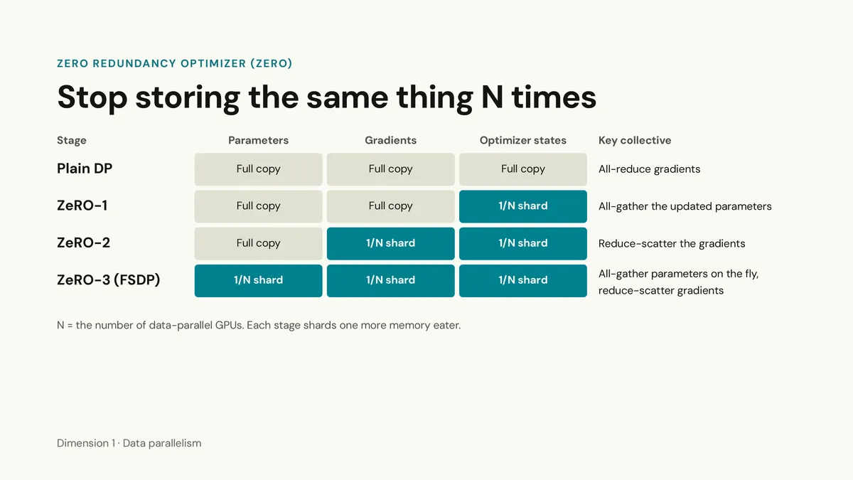
The Zero Redundancy Optimizer (ZeRO) (implemented in DeepSpeed) and FSDP (Fully Sharded Data Parallel, native in PyTorch) eliminate that duplication by partitioning the 20 bytes of state across your $N$ data-parallel GPUs in three stages:

• ZeRO-1 (Optimizer State Sharding): We keep full copies of the BF16 parameters and gradients on every GPU, but shard the bulky FP32 optimizer states ($m,v$, and FP32 master weights) so each GPU only holds $1/N$ of them. At the end of the backward pass, each GPU updates only its $1/N$ slice of parameters, followed by an all-gather so everyone gets the updated BF16 weights. Your forward and backward passes have zero extra overhead compared to DDP, while your memory per parameter drops significantly.
• ZeRO-2 (Gradient + Optimizer Sharding): Since GPU $k$ only updates shard $k$ of the parameters during the optimizer step, it never actually needed the averaged gradients for the other $N-1$ shards. Instead of running an all-reduce on gradients (which equals a reduce-scatter + all-gather), ZeRO-2 stops halfway and just runs a reduce-scatter. Each GPU receives only the averaged $1/N$ gradient slice corresponding to the optimizer shard it owns. This saves even more memory and actually reduces communication slightly compared to naive all-reduce + scatter.
• ZeRO-3 / FSDP (Parameter + Gradient + Optimizer Sharding): Now we shard everything, including the BF16 model weights themselves. At rest, each GPU holds just $1/N$ of the parameters, $1/N$ of the gradients, and $1/N$ of the optimizer state. For an 8B model across 8 GPUs, that 160 GB training state shrinks to just 20 GB per GPU.

Of course, a GPU can't compute the forward pass of Layer 1 on its local data batch if it only has $1/8$th of Layer 1’s weight matrix.

So ZeRO-3 / FSDP materializes each layer on demand:

1. Right before Layer 1 runs in the forward pass, all GPUs execute an all-gather to assemble the full BF16 weights of Layer 1.
2. Every GPU runs the forward pass of Layer 1 on its own local data batch.
3. Immediately after Layer 1 finishes, every GPU frees the $N-1$ weight shards it doesn't own, dropping memory right back down.
4. During the backward pass, it does the same thing in reverse: all-gather the layer weights to compute gradients, free the unowned weights, and reduce-scatter the newly computed gradients.

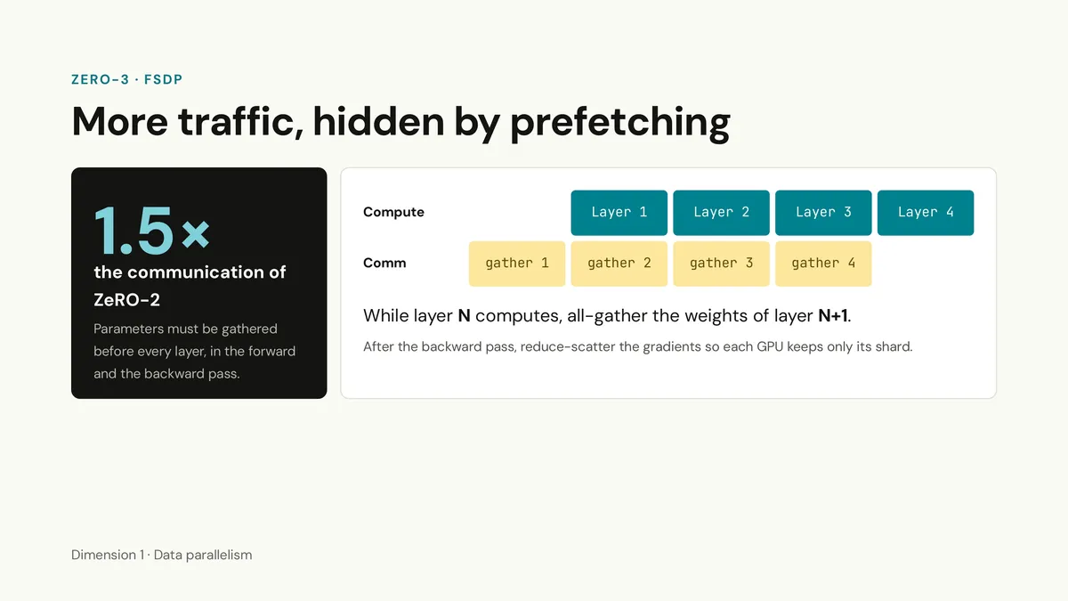
Because ZeRO-3 has to all-gather parameters during both the forward and backward passes (on top of reduce-scattering the gradients), it generates 1.5× the total communication volume of ZeRO-2 or standard DDP.

To keep that extra 50% network traffic from stalling the GPUs, FSDP relies heavily on prefetching: while the compute stream is executing Layer 1, the communication stream is already running gather 2 to pull in the weights for Layer 2 (and in the backward pass, backward_prefetch grabs Layer k-1 while Layer k is still computing).

Practical Realities: What the Slides Don't Tell You About FSDP & ZeRO

Since almost everyone reading this will use ZeRO or FSDP on a weekly basis, there are three practical lessons worth burning into memory before you configure your next run:

1. Never use ZeRO-3 (FULL_SHARD) if ZeRO-2 (SHARD_GRAD_OP) fits in memory. Many practitioners default to ZeRO-3 / full FSDP because "more sharding = less memory = better." In reality, if your model fits under ZeRO-2, switching to ZeRO-3 is pure downside: you pay 50% more network traffic, and if your interconnect can't completely hide the all-gather latency behind compute, your GPU utilization (MFU) drops. Always try ZeRO-2 + activation checkpointing first; only step up to ZeRO-3 when the model genuinely won't fit otherwise.
2. Use Hybrid Sharding (HSDP / ZeRO++) on multi-node clusters. Suppose you have 4 nodes of 8 GPUs (32 GPUs total), and your model needs ZeRO-3 to fit across 8 GPUs. If you run standard ZeRO-3 across all 32 GPUs, every single layer's all-gather has to traverse the slower inter-node network across all 4 servers. Instead, use Hybrid Sharding (ShardingStrategy.HYBRID_SHARD in PyTorch FSDP): it runs ZeRO-3 inside each 8-GPU node (where the frequent weight all-gathers fly over fast NVLink) and plain DDP / gradient all-reduce across the 4 nodes (which only happens once at the end of the gradient accumulation step). On 2-to-8 node setups without top-tier InfiniBand, flipping from FULL_SHARD to HYBRID_SHARD regularly doubles training throughput.
3. Remember that ZeRO-3 does NOT shard activations. ZeRO-3 shards weights, gradients, and optimizer states, plus it still requires enough temporary VRAM buffer to hold one full unsharded layer (or FSDP unit) plus its prefetch buffer during the forward/backward pass. If you wrap your entire model as a single giant FSDP unit instead of wrapping at the TransformerDecoderLayer level, FSDP will all-gather the entire model at once and immediately OOM.

Dimension 2: Tensor Parallelism (Sharding the Math)

What happens when a model is so big that even holding a single unsharded layer and its activations during an FSDP all-gather blows out your memory? Or what if you have hundreds of GPUs and want to cut down both weight memory and activation memory without doing global all-gathers across the whole cluster?

You cut the matrix multiplications themselves. This is Tensor Parallelism (TP), introduced by NVIDIA’s Megatron-LM.

There is one ironclad rule with Tensor Parallelism: keep it inside a single 8-GPU node (TP <= 8). Unlike Data Parallelism (which syncs once per layer or once per accumulation step in the background), TP requires blocking collective communications in the middle of the forward and backward pass of every single layer. Inside a node connected by NVLink (400–900 GB/s bidirectional bandwidth), those syncs take microseconds. Across nodes over Ethernet or standard InfiniBand, latency kills you and your GPUs spend most of their time waiting on the network.

Let's walk through how you split a linear layer $Y=XW$ across two GPUs using concrete numbers.

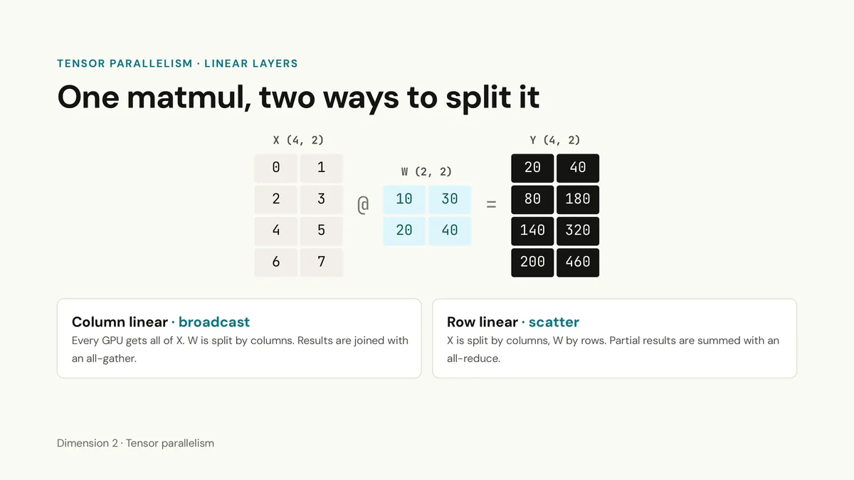
Take an input activation matrix $X$ of shape (4, 2) and a weight matrix $W$ of shape (2, 2):

$X=\left[\begin{array}{cc}0& 1\\ 2& 3\\ 4& 5\\ 6& 7\end{array}\right],W=\left[\begin{array}{cc}10& 30\\ 20& 40\end{array}\right]$

On a single GPU, $Y=X@W$ produces a (4, 2) matrix:

$Y=\left[\begin{array}{cc}20& 40\\ 80& 180\\ 140& 320\\ 200& 460\end{array}\right]$

Now let's split $W$ across GPU 0 and GPU 1. Because a 2D matrix has two axes, there are two ways to slice $W$: along its columns or along its rows.

1. Column Linear: Split $W$ by Columns, Then All-Gather

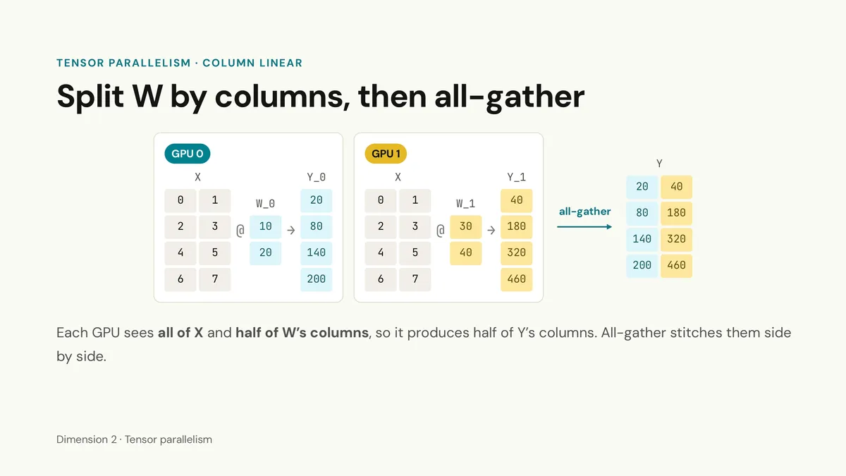
In a Column Linear split, both GPUs receive the full input $X$, and each GPU holds half the columns of $W$:

• GPU 0 holds the left column $W_0=\left[\begin{array}{c}10\\ 20\end{array}\right]$ and computes $Y_0=X@W_0=\left[\begin{array}{c}20\\ 80\\ 140\\ 200\end{array}\right]$.
• GPU 1 holds the right column $W_1=\left[\begin{array}{c}30\\ 40\end{array}\right]$ and computes $Y_1=X@W_1=\left[\begin{array}{c}40\\ 180\\ 320\\ 460\end{array}\right]$.

Because matrix multiplication operates column-by-column on the right-hand matrix, $Y_0$ is already the exact first column of $Y$, and $Y_1$ is the exact second column of $Y$. If we need the full output $Y$ right now, we just run an all-gather to concatenate $Y_0$ and $Y_1$ side-by-side: [Y_0, Y_1] = Y.

2. Row Linear: Split $W$ by Rows, Then All-Reduce

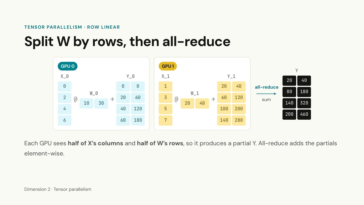
Now suppose we slice $W$ horizontally by rows instead. For the inner dimensions of the matrix multiplication to match, slicing $W$ by rows forces us to slice the input $X$ by columns:

• GPU 0 gets the first column of $X$ ($X_0$) and the first row of $W$ ($W_0=\left[\begin{array}{cc}10& 30\end{array}\right]$). Multiplying (4, 1) @ (1, 2) produces a (4, 2) matrix $Y_0$.
• GPU 1 gets the second column of $X$ ($X_1$) and the second row of $W$ ($W_1=\left[\begin{array}{cc}20& 40\end{array}\right]$), producing another (4, 2) matrix $Y_1$.

Notice the difference: neither $Y_0$ nor $Y_1$ contains final numbers yet. By the block matrix multiplication rule:

$XW=\left[\begin{array}{cc}{X}_0& X_1\end{array}\right]\left[\begin{array}{c}{W}_0\\ W_1\end{array}\right]=X_0{W}_0+X_1{W}_1=Y_0+Y_1$

Each GPU has computed a partial sum of the full (4, 2) output. To get the final $Y$, we run an all-reduce (sum) to add $Y_0$ and $Y_1$ element-wise:

$\left[\begin{array}{cc}0& 0\\ 20& 60\\ 40& 120\\ 60& 180\end{array}\right]+\left[\begin{array}{cc}20& 40\\ 60& 120\\ 100& 200\\ 140& 280\end{array}\right]=\left[\begin{array}{cc}20& 40\\ 80& 180\\ 140& 320\\ 200& 460\end{array}\right]$

Why We Always Pair "Column First, Then Row"

If both Column Linear and Row Linear work, why not just use Column Linear for every layer?

Look at what happens inside a Transformer MLP block, where you have two linear layers separated by a non-linear activation function like GeLU: $\text{MLP}(X)=\text{GeLU}(X{W}^{(1)})W^{(2)}$.

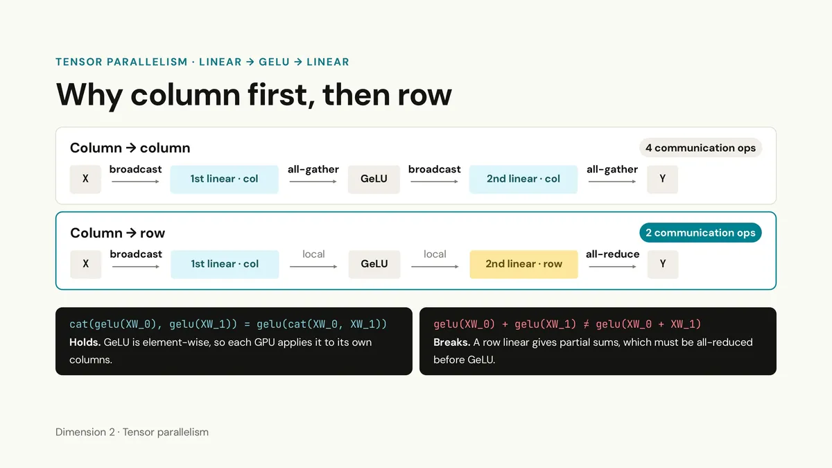
If you use Column $\to$ Column, you have to all-gather the columns after the 1st linear layer, apply GeLU, and then all-gather again after the 2nd linear layer (plus the corresponding backward communications)—totalling 4 communication ops for the block.

Now see what happens when you pair Column $\to$ Row:

1. The first layer is Column Linear. Without doing an all-gather, GPU 0 holds the left columns $X{W}_0^{(1)}$ and GPU 1 holds the right columns $X{W}_1^{(1)}$.
2. Next comes GeLU. Because GeLU acts element-by-element on each scalar independently, applying GeLU to two half-matrices and concatenating them gives the exact same result as concatenating them first and applying GeLU: $\text{cat}(\text{gelu}(X{W}_0),\text{gelu}(X{W}_1))=\text{gelu}(\text{cat}(X{W}_0,X{W}_1))$ That means each GPU can run GeLU locally on its own column slice without any network communication at all.
3. Right after GeLU, GPU 0 holds the left columns of the activated tensor and GPU 1 holds the right columns. And what does a Row Linear layer need as its input? A tensor already split by columns! So the output of GeLU drops straight into the second (Row Linear) layer with zero communication in between.

You only communicate once at the very end of the second linear layer (via the Row Linear all-reduce). That cuts the communication ops in half!

(And you can see on the bottom-right of the slide why Row $\to$ Column doesn't work: a Row Linear layer outputs un-summed partial matrices, and because GeLU is non-linear, $\text{gelu}(A)+\text{gelu}(B)\ne \text{gelu}(A+B)$. You would be forced to run an all-reduce before you could apply GeLU).

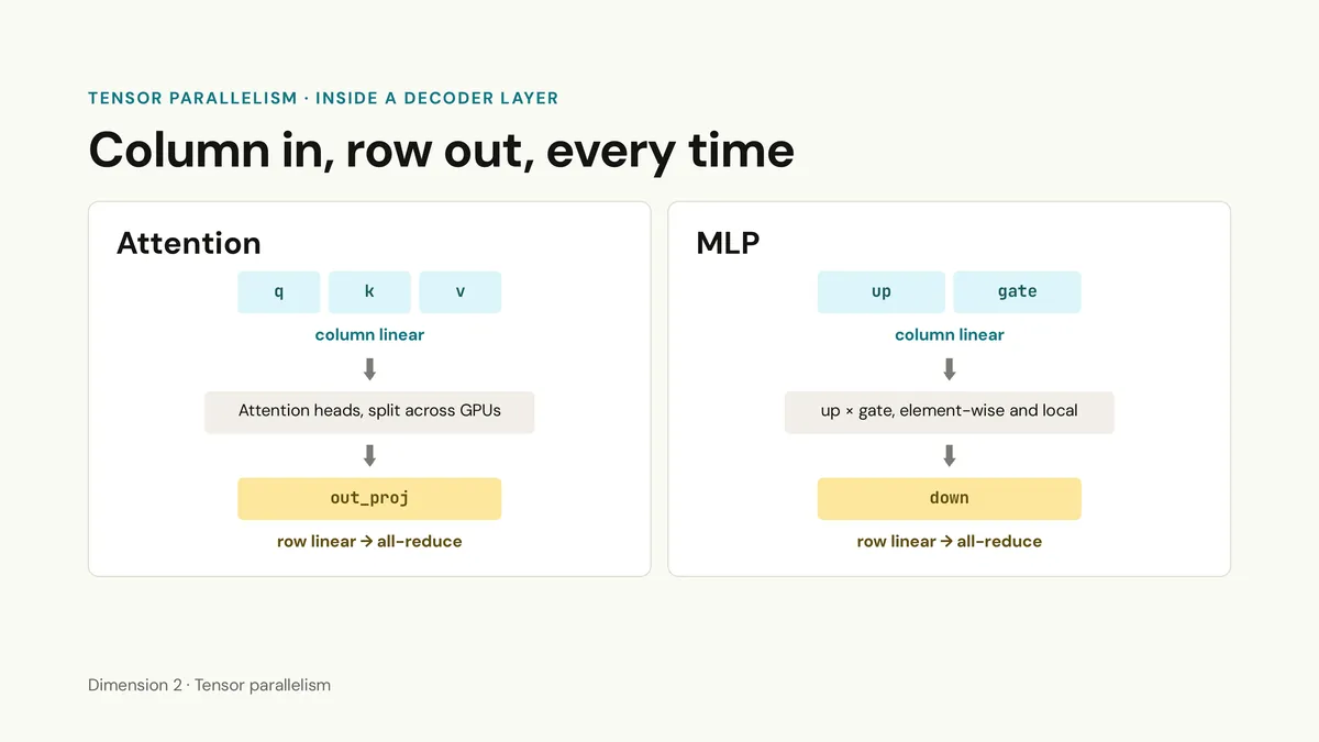
This "Column in, Row out" pattern is the heartbeat of Tensor Parallelism across the entire Transformer decoder layer:

• In Multi-Head / Grouped-Query Attention: The $Q$, $K$, and $V$ projections are Column Linear layers. Slicing $W_Q,W_K,W_V$ by columns cleanly partitions the attention heads across GPUs (for example, with 32 heads across 8 GPUs, each GPU owns 4 heads). Because attention heads don't talk to each other during scaled dot-product attention, each GPU computes FlashAttention on its local heads with zero communication, and then feeds the result into out_proj—which is a Row Linear layer ending in a single all-reduce. (One practical detail for GQA models: if your model has 8 KV heads, you can't easily use TP > 8 without duplicating KV heads across ranks, which is another reason TP = 8 is the natural ceiling).
• In the SwiGLU MLP: Both up_proj and gate_proj are Column Linear. The SiLU activation and element-wise multiplication (silu(gate) * up) happen completely locally on each GPU's column shard, and down_proj is a Row Linear layer ending in an all-reduce.

So across an entire Transformer layer—both Attention and MLP—Tensor Parallelism only needs two all-reduce operations in the forward pass (and two in the backward pass).

Splitting the Embedding Table (Vocab-Parallel Embedding)

Modern tokenizers have huge vocabularies—128,256 tokens in Llama 3, over 150K in Qwen, and 256K+ in multilingual models. At a hidden dimension of 8192, a 128K embedding table plus the output lm_head has over 2 billion parameters by itself. So Megatron also tensor-parallelizes the embedding layer across the vocabulary axis.

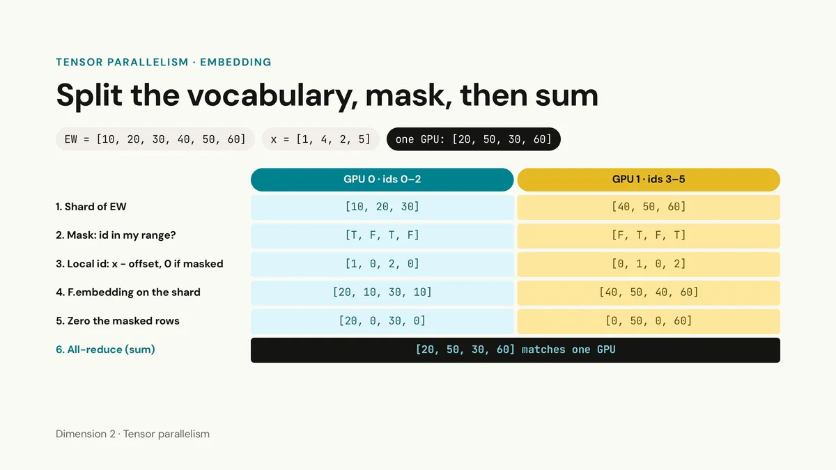
Here is how vocab-parallel embedding works with a toy 1D embedding weight EW = [10, 20, 30, 40, 50, 60] (vocab size 6) and input token IDs x = [1, 4, 2, 5]:

1. Shard the vocab: GPU 0 holds the first half of the vocabulary, IDs 0–2 ([10, 20, 30]). GPU 1 holds the second half, IDs 3–5 ([40, 50, 60]).
2. Build a range mask: Both GPUs receive the full token sequence x = [1, 4, 2, 5] and check which tokens fall inside their local vocab range. GPU 0 gets [T, F, T, F]; GPU 1 gets [F, T, F, T].
3. Shift to local indices: Each GPU subtracts its starting vocab offset (0 for GPU 0, 3 for GPU 1) and clamps out-of-range indices to 0 so F.embedding won't throw an out-of-bounds error. GPU 0 gets local IDs [1, 0, 2, 0]; GPU 1 gets [0, 1, 0, 2].
4. Local lookup: Each GPU runs F.embedding on its local shard. GPU 0 gets [20, 10, 30, 10]; GPU 1 gets [40, 50, 40, 60].
5. Zero out the masked positions: Where the mask from Step 2 was False, overwrite the dummy lookup with zeros. Now GPU 0 has [20, 0, 30, 0] and GPU 1 has [0, 50, 0, 60].
6. All-reduce (sum): Sum the two vectors across GPUs to get [20, 50, 30, 60]—identical to a single-GPU lookup.

Dimension 3: Sequence & Context Parallelism (Sharding the Text)

Tensor Parallelism splits the heavy matrix multiplications inside Attention and MLP, but what happens outside those two blocks?

Between every Attention block and MLP block, you have LayerNorm / RMSNorm, residual connections, and Dropout. Because TP finishes every Attention and MLP block with an all-reduce, the activation tensor exiting that all-reduce is replicated identically on all 8 GPUs.

When sequence lengths were 2,048 tokens, nobody cared that LayerNorm and residual activations were duplicated 8 times inside a node. When you push context length to 32K, 64K, or 128K, those unsharded [batch, seq_len, hidden_dim] boundary tensors become one of the largest consumers of activation memory on the GPU.

Sequence Parallelism (SP): Free Memory with Zero Extra Traffic

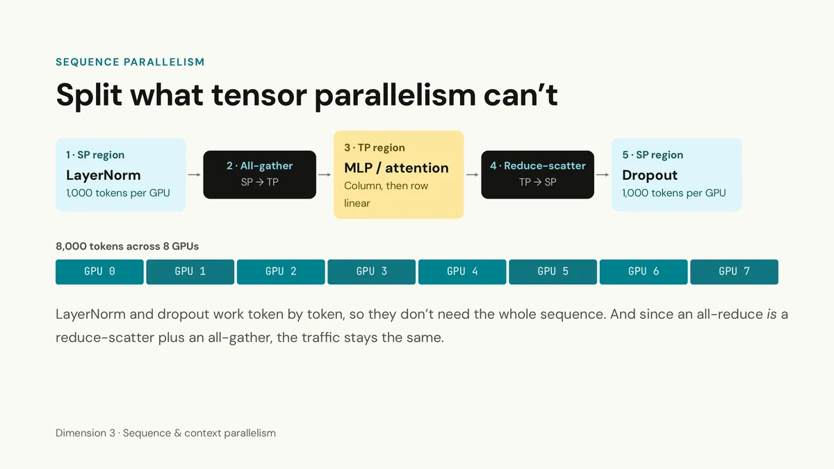
Sequence Parallelism (SP) fixes that duplication by exploiting two facts:

1. LayerNorm, RMSNorm, Dropout, and residual adds are completely independent across the token dimension (seq_len). Computing RMSNorm for token 5 only requires the hidden_dim vector of token 5; it never looks at token 6. So if we have an 8,000-token sequence across 8 GPUs, there is no reason for all 8 GPUs to normalize all 8,000 tokens. Each GPU can just hold 1,000 tokens and normalize its own slice.
2. An all-reduce is mathematically identical to a reduce-scatter followed by an all-gather (and uses the exact same total network bandwidth).

Look at the diagram above to see how SP rewires the layer:

• In standard TP, Step 3 (the MLP or Attention block) ended with an all-reduce that left all 8,000 tokens replicated on every GPU.
• With SP enabled, we replace that all-reduce with a reduce-scatter along the sequence dimension (Step 4). This sums the partial results from the Row Linear layer and splits the 8,000-token sequence into eight 1,000-token chunks in one collective.
• Now we enter the SP region (Step 5 and Step 1 of the next block): each GPU runs Dropout, the residual connection, and the next LayerNorm/RMSNorm on just 1,000 tokens. Activation memory for all these ops drops by $8\times$.
• Right before the next TP Column Linear layer needs the full sequence, we run the second half of our old all-reduce—an all-gather (Step 2)—to reassemble the 8,000 tokens.

Because reduce-scatter + all-gather transfers the exact same number of bytes as a ring all-reduce, turning on Sequence Parallelism alongside Tensor Parallelism is essentially a free lunch: zero extra communication volume, and a massive drop in activation memory. In modern Megatron-style training, TP and SP are almost always turned on together as a pair.

Context Parallelism (CP) & Ring Attention

Here is a question that trips up a lot of engineers: "Wait—if we already use FlashAttention (which avoids materializing the $O(S^2)$ attention matrix) and TP+SP, why do we still run out of memory at 64K or 128K context lengths?"

Because even though FlashAttention makes attention memory linear in sequence length $O(S)$ instead of quadratic $O(S^2)$, linear in $S=128,000$ across 64 or 80 layers is still gigantic! Remember, inside the TP region (Step 3 of the previous slide), we had to all-gather the full sequence of tokens so Attention and MLP could run. Even split 8 ways across heads by TP, holding the $Q,K,V$ projections, MLP intermediate activations (which expand hidden_dim by $3.5\times$ to $4\times$ in SwiGLU), and layer boundary checkpoints for 128,000 tokens inside a single node will blow right past 80 GB per GPU.

To train on ultra-long documents (64K to 1M+ tokens), we cannot all-gather the full sequence anywhere. Every GPU must hold only a $1/N$ chunk of the sequence at all times—even during Attention and MLP. That is Context Parallelism (CP).

In the MLP, LayerNorm, and linear projections, keeping the sequence sharded is trivial because those ops work token-by-token. The only place tokens actually interact with each other is inside Self-Attention, where a Query token at position 100,000 needs to attend to Key and Value tokens all the way back at position 1.

Ring Attention solves this without ever gathering the full sequence on one GPU.

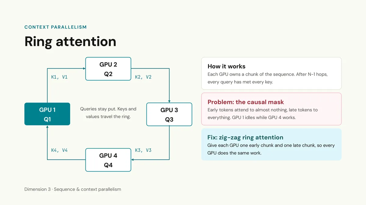
Suppose we split a long sequence into 4 chunks across 4 GPUs placed in a logical ring:

1. Queries stay home: GPU 1 permanently holds $Q_1$, GPU 2 holds $Q_2$, GPU 3 holds $Q_3$, and GPU 4 holds $Q_4$.
2. Keys and Values travel the ring: In Round 0, each GPU computes FlashAttention between its local $Q_i$ and its local $K_i,V_i$. Simultaneously, in the background over P2P network sends/recvs, each GPU passes its $K_i,V_i$ tensor to the next GPU in the ring.
3. In Round 1, GPU 2 now has $K_1,V_1$. It computes attention between $Q_2$ and $K_1,V_1$, merges the result with Round 0's output using online softmax rescaling (the exact same log-sum-exp trick FlashAttention uses across SRAM tiles), and forwards $K_1,V_1$ along to GPU 3.
4. After $N-1$ hops around the ring, every Query chunk has attended to every Key/Value chunk, and each GPU has the exact final attention output for its local sequence chunk.

(A nice practical bonus here: in modern LLMs that use Grouped-Query Attention (GQA), the $K$ and $V$ tensors have $4\times$ to $8\times$ fewer heads than $Q$. Because Ring Attention only sends $K$ and $V$ over the network while keeping the bulky $Q$ tensor stationary, GQA makes it much easier to hide the ring communication completely behind the attention FLOPs!)

The Causal Mask Trap (and How Zig-Zag Ring Attention Fixes It)

If you implement naive Ring Attention for an autoregressive (causal) LLM, you immediately hit a severe load-imbalance bug.

Because of the lower-triangular causal mask, early tokens can only attend to earlier tokens, while late tokens must attend to the entire document:

• If GPU 1 holds tokens 0–32K (the start of the document), its queries $Q_1$ only attend to $K_1,V_1$. When $K_2,K_3$, and $K_4$ (tokens 32K–128K) arrive around the ring, they are completely masked out by the causal mask! So GPU 1 finishes its work in Round 0 and sits idle for Rounds 1, 2, and 3.
• Meanwhile, GPU 4 holds tokens 96K–128K (the end of the document). Its queries $Q_4$ have to attend to $K_1,K_2,K_3$, and $K_4$. GPU 4 does $4\times$ more compute than GPU 1, bottlenecking the entire ring.

The fix is Zig-Zag Ring Attention (striped or symmetric chunking). Instead of cutting the sequence into 4 contiguous blocks, we cut it into $2N=8$ sub-chunks and pair one chunk from the very front with one chunk from the very back on each GPU:

• GPU 1 gets chunks (1, 8)
• GPU 2 gets chunks (2, 7)
• GPU 3 gets chunks (3, 6)
• GPU 4 gets chunks (4, 5)

Because every GPU now holds one early slice (almost no causal work) and one symmetrically late slice (lots of causal work), the total unmasked attention FLOPs on every GPU at every step of the ring are 100% identical. No GPU ever idles waiting for another.

Dimension 4: Pipeline Parallelism (Sharding the Layers)

What if your model has 70B, 405B, or 671B parameters? A single 8-GPU node doesn't have enough memory to hold it, Tensor Parallelism can't leave the 8-GPU node without hitting a latency wall, and running pure ZeRO-3 across 64 or 128 nodes would choke your inter-node network with massive weight all-gathers.

This is where Pipeline Parallelism (PP) comes in. Instead of splitting individual matrices, we assign whole groups of contiguous layers (called stages) to different nodes: Server 1 runs Layers 1–4, sends only the single boundary activation tensor [micro_batch, seq_len, hidden_dim] over the inter-node link to Server 2, and Server 2 runs Layers 5–8.

Because Pipeline Parallelism only communicates point-to-point at the boundary between stages, its network traffic is tiny compared to TP or ZeRO-3. The challenge with PP isn't bandwidth—it's keeping all the GPUs busy at the same time.

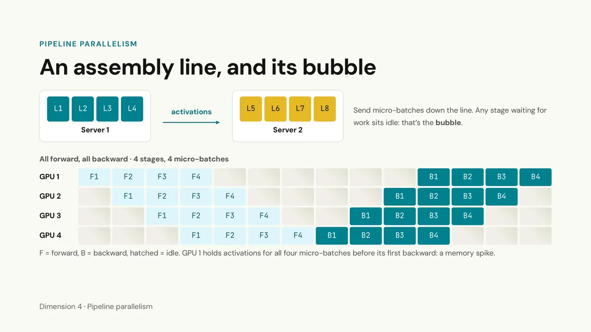
If you feed one big batch into a 4-stage pipeline, Stage 2, 3, and 4 sit completely idle while Stage 1 computes; then Stage 1, 3, and 4 sit idle while Stage 2 computes. Three-quarters of your cluster is wasted.

To fill the assembly line, we split each batch into $M$ smaller micro-batches (F1, F2, F3, F4) and stream them through the stages back-to-back.

The timeline on the slide above shows the simplest schedule, All Forward, All Backward (GPipe). Even with micro-batching, two headaches jump out immediately:

1. The Pipeline Bubble: Look at the gray hatched boxes where stages wait for upstream activations to arrive or downstream gradients to return. The fraction of time spent in that idle bubble is roughly $\frac{P-1}{M}$, where $P$ is the number of pipeline stages and $M$ is the number of micro-batches.
2. The Activation Memory Spike: Look at GPU 1 (Stage 1). It computes forward micro-batches F1, F2, F3, F4 right at the start of the step, and then has to wait for the entire pipeline to finish before it can run its first backward pass B1. That means Stage 1 must hold the forward activations for all $M$ micro-batches in VRAM simultaneously! If you increase $M$ to shrink the bubble, you blow up activation memory on Stage 1.

Four Schedules to Shrink the Bubble

To get around the memory spike and crush that idle bubble, pipeline schedules have evolved through four main generations:

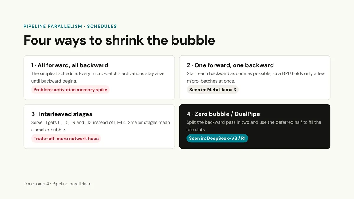
1. All Forward, All Backward (GPipe): Runs all forwards, then all backwards. Easy to reason about, but rarely used in large-scale LLM training today because holding $M$ micro-batches of activations in memory doesn't scale.
2. One Forward, One Backward (1F1B): Instead of waiting for all forward micro-batches to finish, as soon as the last stage finishes F1, it immediately starts B1 and sends gradients upstream. Once the pipeline warms up, every stage alternates strictly between one forward pass and one backward pass (F, B, F, B...). Because each B immediately frees the saved activations of a prior F, peak in-flight activation memory on Stage 1 is capped at $P$ micro-batches instead of $M$—letting you crank up $M$ to shrink the bubble without running out of memory. (Meta used 1F1B to train Llama 3 405B).
3. Interleaved 1F1B: Instead of giving each server one big block of contiguous layers (Server 1 = L1–L4, Server 2 = L5–L8), you assign each server multiple smaller "virtual stages" looped around the pipeline (Server 1 = L1–L2 and L9–L10). Because each micro-batch passes through smaller chunks of layers faster, the pipeline warms up and drains much quicker, reducing the bubble size by a factor of $v$ (the number of virtual stages per GPU), at the cost of $v\times$ more point-to-point network hops.
4. Zero Bubble & DualPipe: Popularized by Sea AI Lab's Zero Bubble paper and pushed to production scale in DeepSeek-V3 and DeepSeek-R1 (via their bidirectional DualPipe schedule, which also overlaps forward/backward compute with MoE all-to-all communication).

How do you get a pipeline bubble down to zero without changing the math of backprop?

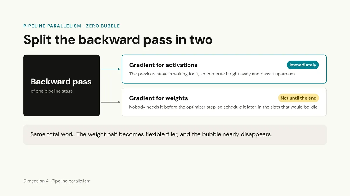
When we draw B1 on a pipeline diagram, we treat the backward pass of a layer $Y=XW$ as a single monolithic block. Under the hood, though, the backward pass of every linear layer is actually two completely separate matrix multiplications:

1. Gradient with respect to input activations ($dX=dY·W^T$, often called $B$): Stage $k-1$ upstream cannot start its own backward pass until Stage $k$ computes $dX$ and sends it back over the network. So $dX$ is on the critical path and must be computed immediately.
2. Gradient with respect to weights ($dW=X^T·dY$, often called $W$): Who is waiting on $dW$? Nobody. No upstream stage needs $dW$. The only thing that ever touches $dW$ is the local optimizer step (optimizer.step()) at the very end of the entire batch!

Zero Bubble schedules un-fuse the backward pass into those two distinct operations: $B$ (activation grad) and $W$ (weight grad). During the main pipeline flow, each stage only computes $B$ and immediately fires $dX$ upstream so the previous stage never has to wait. Meanwhile, all those $W$ matmuls are placed into a local work queue. Whenever a GPU hits an idle "bubble" slot where it is waiting for the network, it pops a deferred $W$ matmul off the queue and computes it to fill the gap. Same exact FLOPs, same exact gradients, and the idle bubble practically disappears.

Dimension 5: Expert Parallelism (Sharding the Experts)

In the live talk, Expert Parallelism only got one slide because of time constraints. In practice right now, though, you can't talk about frontier LLM training without talking about Mixture-of-Experts (MoE). From Mixtral to Qwen-MoE to DeepSeek-V3/R1, MoE has become the dominant way to scale model capacity without blowing up per-token compute FLOPs.

In a dense Transformer, every single token passes through the exact same giant Feed-Forward (MLP) network. In an MoE layer, you replace that single giant MLP with $E$ smaller parallel MLP sub-networks called experts (for instance, 8 experts in Mixtral 8x7B, or 256 routed experts in DeepSeek-V3) plus a tiny linear router (gating network). For each incoming token, the router outputs a probability distribution over all experts and selects only the top-$k$ experts to actually process that token.

This creates an interesting systems problem: a model like DeepSeek-V3 has 671B total parameters (so all the experts combined require massive amounts of VRAM), yet each individual token only activates 37B parameters ($k=8$ out of 256 routed experts).

Expert Parallelism (EP) distributes those experts across GPUs:

• If you have 64 experts and 8 GPUs (EP = 8), GPU 0 holds Experts 0–7, GPU 1 holds Experts 8–15, and so on.
• Attention layers stay replicated (Data Parallel) or Tensor Parallel as usual.
• When tokens reach an MoE layer, each GPU runs the router locally on its tokens. Suppose GPU 0 has a token "apple" that the router assigns to Expert 12 (which lives on GPU 1), and a token "code" assigned to Expert 60 (which lives on GPU 7).
• All GPUs in the EP group execute an all-to-all collective (token dispatch) to physically ship each token's hidden state over the network to whichever GPU hosts its chosen expert.
• Each GPU runs its local experts on the batch of tokens it just received from across the cluster.
• Finally, the GPUs execute a second all-to-all collective (token combine) to send the processed token vectors back to their original home GPUs, where they are weighted by the router probabilities and added back to the residual stream.

Three Practical Headaches with Expert Parallelism

If you ever train or fine-tune an MoE model with Expert Parallelism, you will immediately run into three systems quirks that don't exist in dense models:

1. The "Hot Expert" Straggler Problem (Load Imbalance): In Data, Tensor, Sequence, and Pipeline Parallelism, every GPU knows ahead of time exactly how many tokens and FLOPs it will compute. In Expert Parallelism, the workload is data-dependent and dynamic! What if, on a given batch of Python code, the router decides to send 80% of all tokens across the entire cluster to Expert 12 on GPU 1 (the "coding expert"), while sending almost nothing to the experts on GPU 4? GPU 1 gets buried in compute (or even OOMs from holding too many incoming token activations), while the other 7 GPUs sit completely idle waiting at the second all-to-all barrier.
   • How we fix it: During training, MoE models use auxiliary load-balancing losses (or auxiliary-loss-free dynamic bias terms, as introduced in DeepSeek-V3) that nudge the router to distribute tokens evenly across experts. Many frameworks also set a hard capacity factor (dropping overflow tokens through the residual connection if an expert's buffer fills up) or use dropless MoE (dMoE / MegaBlocks) with block-sparse matrix kernels to handle variable-sized token buckets without padding waste.
2. All-to-All Is Brutal on Network Topology: In an all-reduce or reduce-scatter, communication can be neatly pipelined around a ring. In an all-to-all, every GPU in the EP group simultaneously talks to every other GPU in the EP group twice per layer (once in dispatch, once in combine, and again in backward!). If your EP degree spans across multiple nodes with oversubscribed network switches, all-to-all congestion will tank your throughput unless you use hierarchical routing (restricting a token to pick experts on at most $M$ nodes) or overlap the all-to-all with compute (like DualPipe does).
3. Shared Experts vs. Routed Experts: Modern MoEs (like DeepSeek and Qwen) often split their experts into 1 or 2 "shared experts" (which process every token deterministically, just like a dense MLP) plus dozens of routed experts. In your parallelism config, those shared experts don't need all-to-all routing—they stay replicated on each GPU (or sharded via Tensor Parallelism), and their computation can actually be overlapped on a separate CUDA stream while the routed tokens are flying across the network in the all-to-all!

Putting It All Together: The 5D Cheat Sheet

Let's zoom out and put all five dimensions on one table so you can see how they fit together.

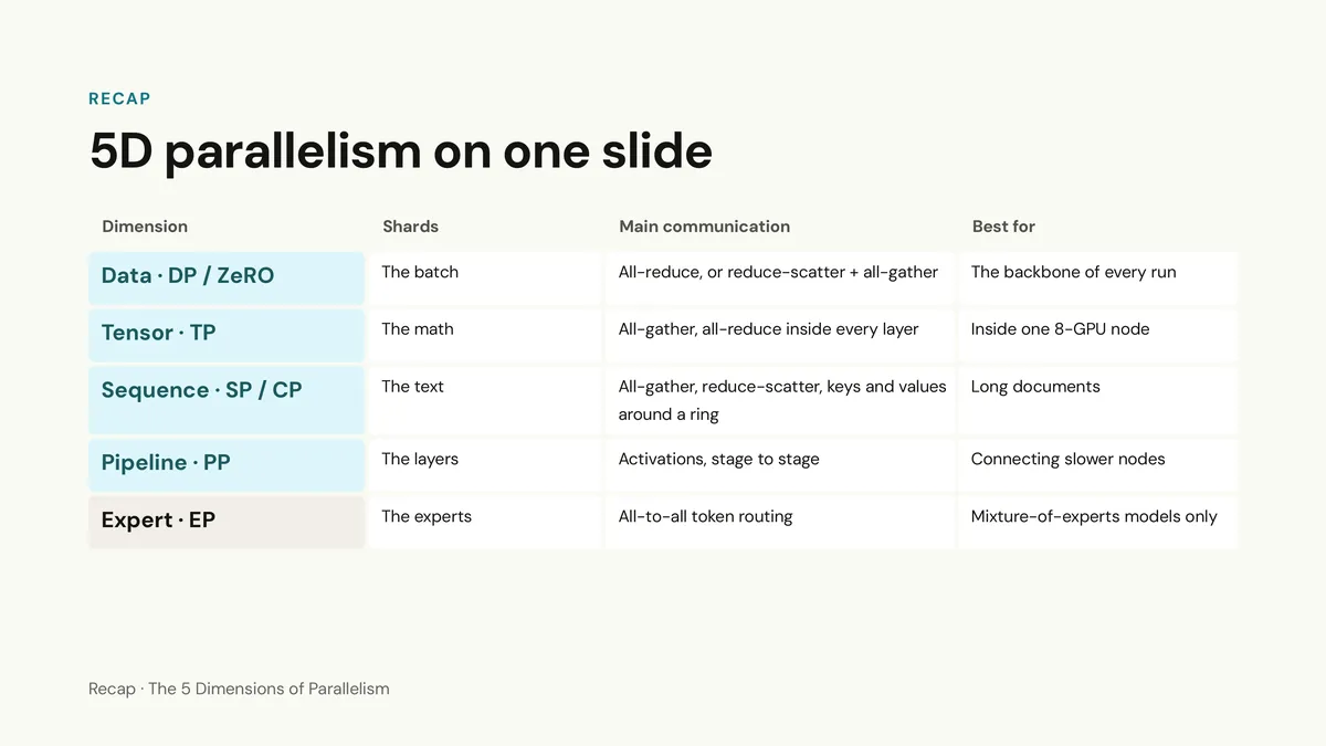
Notice how orthogonal they are:

• Data Parallelism (DP / ZeRO / FSDP) slices the batch (and shards model state), communicates via all-reduce or reduce-scatter + all-gather, and scales out throughput to any number of GPUs.
• Tensor Parallelism (TP) slices hidden_dim, communicates via all-reduce inside every layer, and stays strictly inside a single 8-GPU NVLink node.
• Sequence & Context Parallelism (SP / CP) slices seq_len, communicates via reduce-scatter/all-gather (SP) or ring P2P transfers of $K,V$ (CP), and keeps long-context activations from exploding.
• Pipeline Parallelism (PP) slices layers, communicates small boundary activations point-to-point between stages, and spans across multiple nodes when a model is too big for one server.
• Expert Parallelism (EP) slices experts, communicates via all-to-all token dispatch/combine, and scales parameter counts in MoE models.

When you combine them on a large cluster, the total number of GPUs in your job is simply the product of your parallel degrees: $\text{Total GPUs}=\text{DP}\times \text{TP}\times \text{CP}\times \text{PP}$ (With Expert Parallelism typically folding into or replacing a subset of the DP/TP axes specifically for the MoE MLP layers: ${\text{DP}}_{\text{expert}}\times \text{EP}={\text{DP}}_{\text{attention}}$).

Pick Your Recipe: What Should You Actually Run?

In practice, you never turn on all five dimensions just to look clever. Every additional parallelism dimension introduces communication overhead, extra process groups, checkpointing headaches, and potential bugs. Your goal isn't just "make the OOM error go away"—it's maximizing MFU (Model FLOPs Utilization), the percentage of theoretical peak GPU compute you're actually achieving.

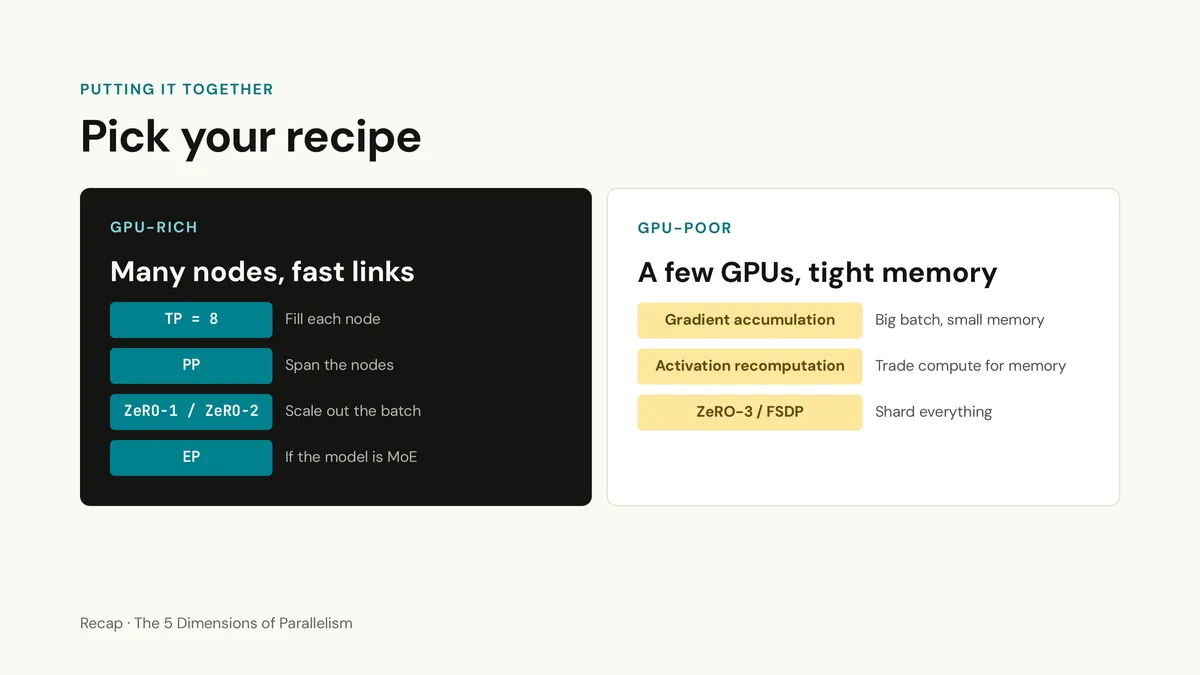
On the slide above, I split the world into GPU-Rich and GPU-Poor. In the real world, I find it helps to break that down into three concrete hardware tiers:

Tier 1: The "GPU-Poor" Single Node (1 to 8 GPUs, e.g., Fine-Tuning 7B–70B)

If you are working on a single node of 2, 4, or 8 GPUs (A100s, H100s, or L40Ss) doing SFT, DPO, or continued pre-training:

• Start with ZeRO-2 or ZeRO-3 (PyTorch FSDP / DeepSpeed) across your GPUs. Because all your GPUs are on the same machine, even ZeRO-3’s extra all-gather traffic stays local and fast.
• Turn on Activation Recomputation (gradient checkpointing) and FlashAttention-2/3. This is non-negotiable for keeping activation memory sane.
• Use Gradient Accumulation (wrapped in no_sync()) to hit your target effective batch size while keeping micro-batch size small (1–4 sequences per GPU).
• Pack your sequences (concatenating short examples together with a block-diagonal cu_seqlens mask instead of right-padding every short sequence with <pad> tokens out to max_seq_len). In fine-tuning, sequence packing often gives a bigger speedup than any parallelism tweak because you stop doing matmuls on pad tokens!
• Do you need TP or PP here? Almost never for training 7B–32B models on a single node—FSDP + activation checkpointing is simpler and usually faster.

Tier 2: The "Awkward Middle" (2 to 8 Nodes / 16 to 64 GPUs)

This is where most startup and enterprise ML teams live, and it's where the most performance gets left on the table. You have a handful of nodes, maybe connected by standard cloud networking (RoCE / TCP / EFA) rather than a dedicated non-blocking InfiniBand fabric:

• First choice: Hybrid Sharding (HSDP / ZeRO++). Shard weights with ZeRO-3 inside each 8-GPU node (shard_group = 8), and replicate / all-reduce gradients across the nodes (replicate_group = num_nodes) at the end of several gradient accumulation steps. This keeps all the chatty weight all-gathers inside the fast NVLink domain and barely touches the inter-node network.
• If the model is 70B+ or sequence length is 32K+: Add TP = 4 or 8 (with SP) inside each node so a single node doesn't choke on activation memory, and wrap ZeRO-1 or ZeRO-2 across the nodes.
• If your context length hits 64K–128K+: Turn on Context Parallelism (CP = 2 or 4) using Zig-Zag Ring Attention so no single GPU has to hold the full sequence activations.

Tier 3: The "GPU-Rich" Pre-Training Cluster (16 to 1,000+ Nodes, Fast InfiniBand)

When you are pre-training a 70B+ dense model or a several-hundred-billion-parameter MoE across hundreds or thousands of GPUs:

• Inside each node: Lock in TP = 8 + SP over NVLink.
• Across nodes (Model Depth): Use Pipeline Parallelism (PP) with a 1F1B, Interleaved 1F1B, or Zero-Bubble/DualPipe schedule so the model spans across nodes with minimal point-to-point activation traffic.
• Long-context stage: Add CP across fast links when extending context windows to 128K+.
• For MoE models: Carve out Expert Parallelism (EP) across high-bandwidth groups for the MoE layers, overlapping the all-to-all dispatch/combine with shared-expert or backward-pass compute.
• Outer loop (Batch Scaling): Wrap the entire multi-node pod in Data Parallelism with ZeRO-1 (or ZeRO-2) to scale out the global batch size to millions of tokens per step without paying the 1.5× inter-node communication tax of ZeRO-3.

When you strip away the acronyms, every single distributed training system out there—whether it's Megatron-LM, DeepSpeed, PyTorch FSDP2, or TorchTitan—is just choosing which axis of [batch_size, seq_len, hidden_dim, layers, experts] to slice, and scheduling the resulting all-gather, reduce-scatter, all-reduce, or all-to-all collectives so the network card is working while the Tensor Cores are busy.

If you're currently wrestling with a multi-node training setup, hitting weird OOM spikes on long sequences, or trying to squeeze higher MFU out of your GPUs, feel free to reach out on LinkedIn or drop a comment below. Always happy to talk shop!

#distributed-training #gpus #llm #machine-learning #parallelism